In the regime of over-parameterized pretrained models, task-specific adaptation proves tricky at scale. The classical full fine-tuning approach of optimizing the entire model and storing the complete set of weights for each task is just prohibitive given the computational and memory requirements. And for students/hobbyists, consumer hardware can’t keep up with the trend of “throw more data at a bigger transformer”.

Thankfully, there is a host of techniques categorized as parameter-efficient fine-tuning methods, or PEFT, that are working to democratize the custom model. After considerable work in prompt tuning and adapter modules, a breakthrough of sorts came in the form of LoRA: Low-Rank Adaptation of Large Language Models¹

For context, previous findings ^{2 3} have illustrated the low intrinsic dimension that typical over-parameterized pretrained weight matrices tend to reside on. In other words, large pretrained models empirically have some lower-dimensional subspace that captures enough of the objective landscape to enable optimization, so it’s possible to restrict the dimensionality of our parameter space during fine-tuning without degrading performance.

By analogy, imagine navigating down a hyperdimensional mountain range by always heading for the steepest slope. You might worry you’ll end up stuck in a hole where every direction is up, but soon you’ll find every valley is actually a saddle point, and the real danger is running out of steam in your meandering descent through them. It might be helpful to use a map! Using an \(r\)-D projection of the landscape (where \(r\) is small) could help prune your options and identify a more direct route down. But if \(r\) is too low, you’re cooked (imagine how helpful a 1-D hiking map would be).

This leads us to LoRA, where we approximate the incremental update \(\Delta W\), i.e. the accumulated gradient steps to the pretrained model from fine-tuning, using a low-rank matrix decomposition. Explicitly, for a pretrained weight matrix \(W_0 \in \mathbb{R}^{d \times k}\), we can reparameterize as:

\[W = W_0 + \Delta W = W_0 + BA\]

with \(B \in \mathbb{R}^{d \times r}\), \(A \in \mathbb{R}^{r \times k}\), and \(r << min(d, k)\). By leaning on the assumption that \(W_0\) has a low intrinsic dimension (meaning the update \(\Delta W\) should have a low “intrinsic rank”), we enforce the bottleneck dimension of \(r\) on \(\Delta W\) and only optimize the parameters of \(BA\).

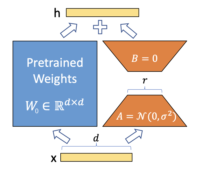Figure 1: LoRA Reparameterization

The benefits of this approach are threefold. First, we’ve gone from \(d \times k\) trainable parameters per module to \((d + k) \times r\). Depending on the scale of our model and our selection for \(r\) (e.g., \(r = 8\) for \(d = k = 1024\)), this can be as dramatic as a \(1000\)x reduction in parameter count! Second, as opposed to previous adapter methods, this approach incurs no additional inference cost. At deployment, we can compute and store \(W = W_0 + BA\), use \(W\) as usual, then efficiently update \(W\) as \(W' = W - BA + B'A'\) to switch to a new downstream task.

And third, there are empirical cases for LoRA outperforming full fine-tuning!

This last point is a seemingly incredible result, but must be taken with the understanding that flashy numbers from arxiv tables are not always representative of real-world performance. We can’t always expect a low-rank matrix to have enough functional expressability to capture the objective landscape. For example, imagine we pretrain with language data and fine-tune on a vision task; full fine-tuning would crush LoRA. It has something to do with the relationship between intrinsic dimension and task difficulty, as well as how well the resultant embedding space after pretraining translates analogical relationships, semantic proximity, and some inexpressible gestaltung hierarchy into cosine similarities and euclidean distances. As much as we try to visualize and understand these embeddings with techniques like t-SNE, our ability to conceptualize higher-dimensional spaces is severly limited by our 3D-oriented neural hardware. The advent of deep learning seemingly necessitates rapid progress here, but more on that in a future post.

Back in the PEFT realm, AdaLoRA⁴ is a technique that drops the LoRA decomposition in favor of an SVD-flavored adaptation that iteratively prunes singular values based on their “importance”. A helpful parallel to consider is the role of the SVD in dimensionality reduction techniques (namely principal-component analysis) and the separable models perspective. The new reparameterization becomes:

\[W = W_0 + \Delta W = W_0 + P \Lambda Q\]

where \(P \in \mathbb{R}^{d \times r}\), \(Q \in \mathbb{R}^{r \times k}\), \(\Lambda = \text{diag}({\lambda_i}, \ 1 \leq i \leq r)\), and again \(r << min(d, k)\). It’s important to note that we aren’t actually calculating the SVD of the updates; rather, we enforce the orthogonality of \(P\) and \(Q\) (using the following regularization term) and trust our SVD intuition applies to the tuned \(\lambda_i\) values. The regularization is simply:

\[R(P,Q) = \|P^\top P - I\|_F + \|QQ^\top - I\|_F\]

We can update \(P\) and \(Q\) in the standard gradient descent fashion, but pruning \(\Lambda\) takes some additional steps. We first calculate \(S^{(t)}\), the “importance” score of all triplets (i.e. all \(\lambda_i\) values and their singular vector equivalents), then update \(\Lambda\) as:

\[\Lambda^{(t+1)}_k = \mathcal{T}(\tilde{\Lambda}^{(t)}_k, S^{(t)}_k), \text{ with } \mathcal{T}(\tilde{\Lambda}^{(t)}_k, S^{(t)}_k)_{ii} = \begin{cases}\tilde{\Lambda}^{(t)}_{k, ii} & S^{(t)}_{k, ii} \text{ is in the top-}b(t)\text{ of } S^{(t)}, \\ 0 & o.w. \end{cases}\]

noting that \(b(t)\) denotes our parameter budget at timestep \(t\) (can also think of \(b(t)\) as the “total rank” of our incremental matrices). This is a lot of fun notation to say each timestep we mask out the values of the post-gradient step \(\tilde{\Lambda}^{(t)}\) at layer \(k\) that fall outside our shrinking budget, ranked by their sensitivity to the training loss with some smoothing!

For a more comprehensive mechanistic illustration, the original AdaLoRA paper is very well explained, but for the purposes of this post it may be helpful to continue on to what this all means.

LoRA and AdaLoRA both take advantage of the following realizations:

1. The modules of pretrained models tend to have a low intrinsic dimension, meaning we can still reach the solution manifold while navigating a lower-dimensional subspace of the objective landscape.
2. We can capitalize on this by reparameterizing the accumulated update to our pretrained weights as low-rank matrices.
3. Not all parameters are created equal. Given a fixed budget, we should maximize the effect of our incremental updates through selective application across layers and modules.

The main difference between LoRA and AdaLoRA is the amount of effort/framework engineering going into this last point. We can build some more intuition for this by thinking about contextualized embeddings in deep nets. It’s a well-established result that embedding quality increases (almost) monotonically alongside model depth. We can see this in the figure below (thanks Jay), which compares performance across six embedding choices:

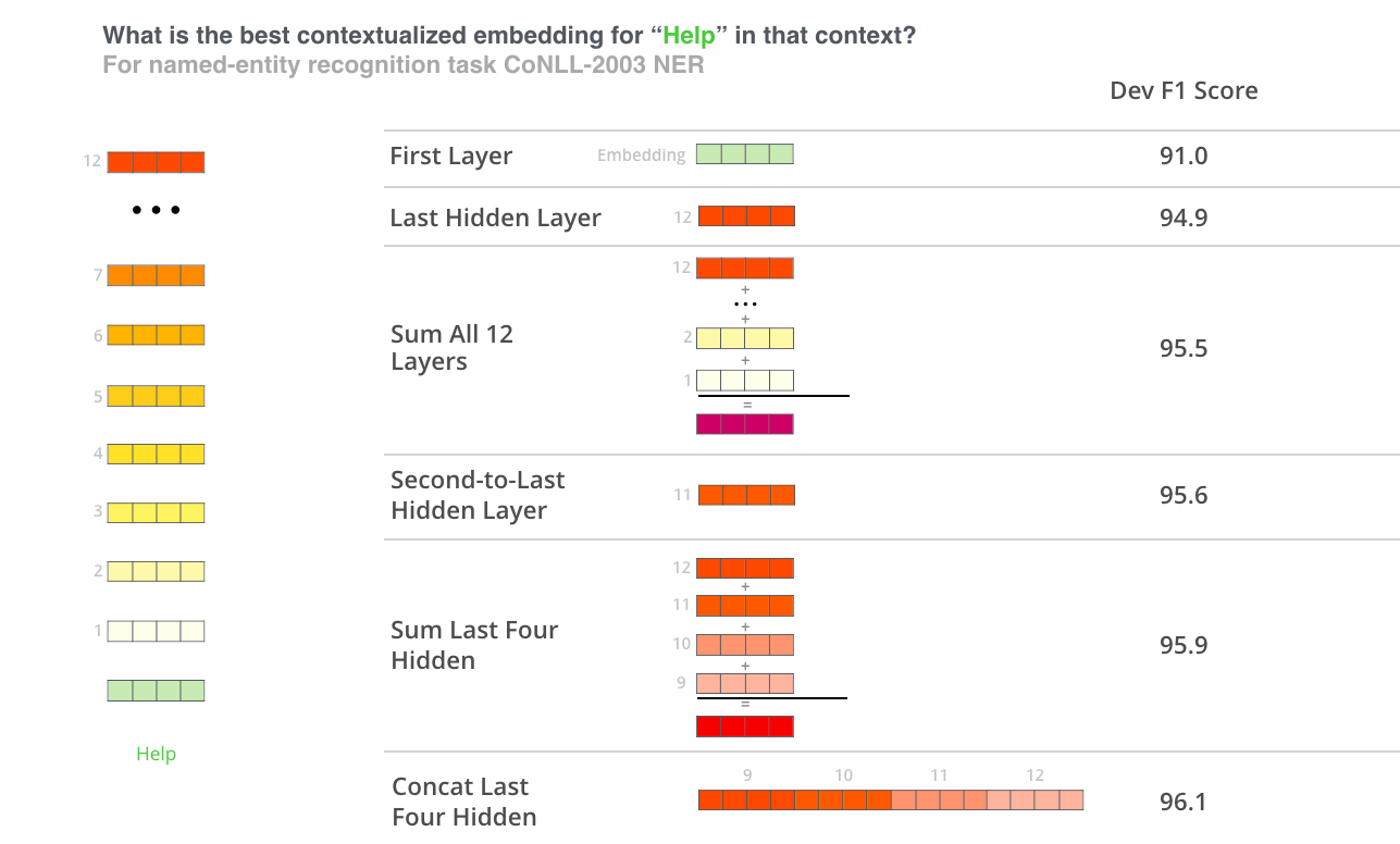Figure 2: Feature-based NER Ablation Results

We can hypothesize that earlier layers are responsible for capturing local features of the input data, while deeper layers are increasingly abstract and capture more complex or global relationships. As it propagates, the representation can gain hierarchical and nuanced features by incorporating dependencies from a broader context. However, the results show the second-to-last layer achieved the best single-layer performance, which could imply that the last layer is more aligned to the surrogate task and contains less general information.

As a quick exercise, use this info to try and guess what the AdaLoRA ablations revealed about fine-tuning importance regarding early layers vs deep layers and attention modules vs feed-forward networks.

As expected considering the results above, deep layers held a stronger impact on performace when fine-tuned over early layers. However, the comparison between attention modules and feed-forward nets may be a little murkier. According to their ablations, the feed-forward nets were preferred!

As a mental framework for this result, we can think of each transformer block being split into two components: a feature generator (captures dependencies, contextualizes representations, dynamically weights input segments) and an inference engine (transforms & refines input while injecting non-linearities). The attention module, the feature generator, learns these less-domain specific abilities during pretraining. And the feed-forward network, the inference engine, moves from these features to something more aligned with the downstream task. As a toy example, we can imagine how adjective-noun association is agnostic to whether you are doing translation or sentiment analysis. To be clear, full-finetuning does benefit from optimizing both. But generally, when operating under time/compute restrictions, a blanket “update everything generically” is just lazy.

Deep nets are not just soups of homogenous weights. Taking care to understand their mechanisms and building algorithms in light of them is at the core of PEFT and the democratization of model training.

P.S. I’m excited to read Mount Analogue: A Tale of Non-Euclidean and Symbolically Authentic Mountaineering Adventures (ty Shaye), will revisit this post after.

1. Hu et al., LoRA: Low-Rank Adaptation of Large Language Models, 2022 ↩

2. Li et al., Measuring the Intrinsic Dimension of Objective Landscapes, 2018 ↩

3. Aghajanyan et al., Intrinsic Dimensionality Explains the Effectiveness of Language Model Fine-Tuning, 2020 ↩

4. Zhang et al., AdaLoRA: Adaptive Budget Allocation for Parameter-Efficient Fine-Tuning, 2023 ↩